MOTIVATION
Check our Youtube video as a quick overview of the project.
Surveillance Video Extraction
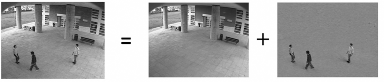
Our project was motivated by surveillance video extraction. In real world, it is often desirable to decompose a video into its background and people in the foreground. Let us represent a video by a matrix, where each column contains the pixel information of one frame and all the frames are stacked column by column. Since the background is often static without any change over frames, it can be thought as an underlying low-dimensional structure. The changing scenario in the foreground, say people walking around, are noises imposed on that. A Robust Principal Component Analysis (Robust PCA) catches such pattern for a matrix M, decomposing it as the sum of a low-dimension matrix L and a sparse matrix S. Candès [3] showed that it can be achieved by solving:
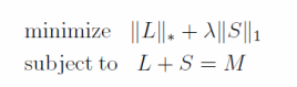
where the underscored '*' represents the nuclear norm taking care of the rank of L and '1' the L1 norm restricting the sum of non-zero terms of S.
Although the Robust PCA can be solved by being converted into a convex optimization problem, finding a computationally efficient algorithm takes a long way. The interior point method, serving as an immediate solution, takes O(n^6) complexity on choosing step directions, thus unfeasible for large problems. In 2009, [5] and [7] proposed an alternating directions method using augmented Lagrange multiplier. The algorithm is much more efficient with O(n^3) complexity, however still suffers from a bottleneck of taking SVD decomposition for the video matrix as pointed out by [2].
Bonus for Video Data: From SVD to QR
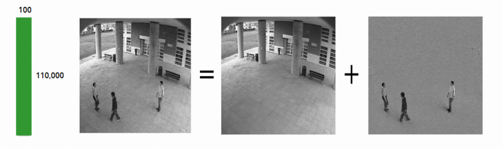
The SVD for video matrix is an unique challenge in that the matrix is usually tall and skinny. In the example above, a single frame, represented by a column, contains 110,000 pixels while only a total of 100 frames are available. We can take advantage of this structure by converting the large SVD to a large QR and a subsequent tiny SVD, as illustrated below.
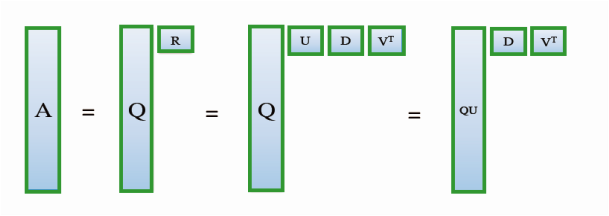
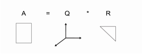
Firstly, we conduct a QR factorization on the tall-skinny matrix A, resulting in a tall-skinny column-orthogonal matrix Q bearing the same shape of A and a small upper-triangular square matrix R. Then a further SVD is done on R, giving us orthogonal matrices U and V, plus a diagonal D. We can immediately observe that the product of Q and U is also orthogonal. Therefore, by simply multiplying Q and U, we get a valid SVD of A.
In practice, as long as we get R, the SVD decomposition of A can be obtained without Q, since the left-singular matrix QU can be calculated via the right-singular matrix V, the singular-values stored in D, and the original matrix A. Going one step further, we can even get Q backwards from QU as the inverse of an orthogonal U is just its transpose. These features enable great flexibility in real-world computation.
Based on these observations, we focus our work in this project on the large QR.
Parallel Tall-Skinny QR on a Binary Tree
Mathematically, a QR decomposition to an arbitrary-size matrix A factorizes it into a column-wise orthogonal matrix Q and an upper-triangular matrix R. A parallel TSQR algorithm takes advantages of A's tall-skinny shape. Below we will walk the algorithm through.
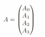
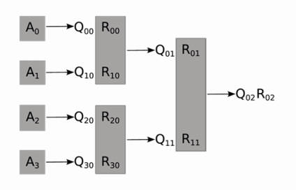
The basic idea is to use a reduction on a binary tree. We adopt the notations of [4]. For a parallel system of P = 4 processors, we divide the m * n matrix A into four (m/4) * n blocks at the first step. Then, four QR factorization are computed independently on four nodes.
|
|
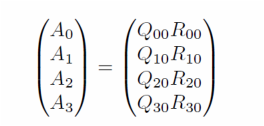
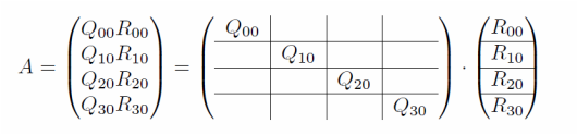
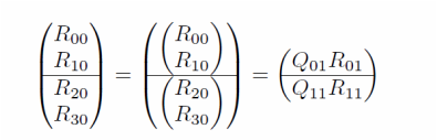
For the subscripts, the Fortran convention is used so that the first index changes more frequently than the second. From the second subscript 0 of Q and R's, we can tell this is the "stage 0" of the computation. The first subscript, ranging from 0 to 3, indicates the block index. This decomposition can also be written in the form of block-wise matrix multiplication as below.
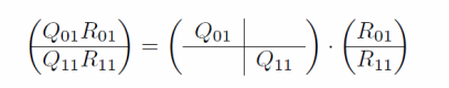
We group the four R factors acquired from stage 0 into two successive pairs, with a QR decomposition on each pair again in parallel. The block-wise form is shown.
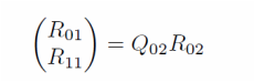
Lastly, the two R factors in stage 1 are combined. A final QR is conducted. The R_02 here is the root of the tree, also the final R for matrix A.
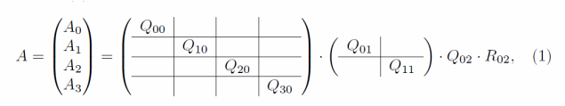
Here is the whole factorization process, in which the product of the first three matrices forms Q, while the R_02 is the R. One can tell that the calculation of Q is fairly challenging in the parallel setting due to the irregular communication structure as well as matrix stacking. Our Design section stage 3 discussed this in detail. Although it has been pointed out earlier in this Motivation that the explicit formation of Q is not always necessary and can be bypassed via mathematical techniques, we still implemented the Q part in our applications as a complete realization of the whole algorithm.
The binary tree structure is shown below.
CS 205 Final Project | Fall 2013 | Xueshan Zhang and Ming Zhu
