PERFORMANCE
We analyzed our performance by comparing four pairs of algorithms. The first comparison was between the serial and GPU realizations of the householder QR algorithm. From the second comparison, we studied the speedup brought by TSQR. We implemented the binary tree (i.e. the TS part) by MPI, altering the methods to compute the QR for each local block. Numpy QR was tested at first, followed by our self-implemented serial QR. The CUDA QR was the last.
Due to the limit of the Harvard resonance cluster, we were not able to load the CULA module for a further performance comparison, which could be interesting as we would like to see if we can replicate the result in [1].
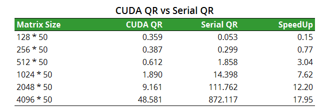
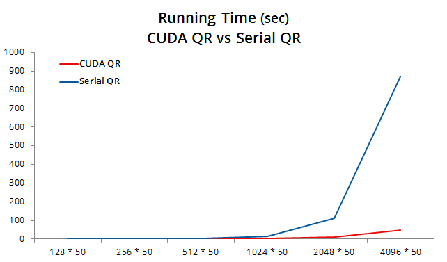
1. Householder QR: CUDA vs Serial
As documented in Application, a matrix with entry number larger than or equal to 8192 * 100 will not be able to be processed due to the memory limit of GPU C2070. Here we chose the column number of 50 and increase the row size from 128 to 4096.
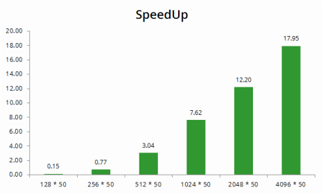
The CUDA QR enjoys a growth of speedup as the matrix size increases. For the largest matrix below with size 4096 * 50, we observe a speedup of 18×.
The CUDA QR enjoys a growth of speedup as the matrix size increases. For the largest matrix below with size 4096 * 50, we observe a speedup of 18×.
|
|
2. TSQR: MPI + Numpy vs Numpy
From this part, we analyze the speedup and efficiency under distributed-memory computing environment. Firstly we compare the performance of serial Numpy QR and MPI Numpy QR.
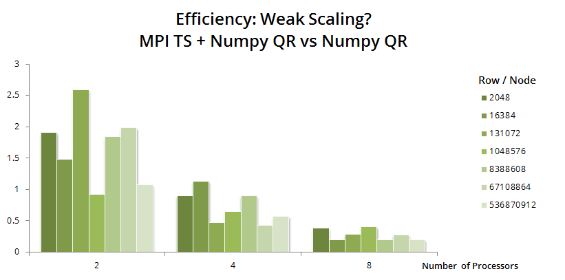
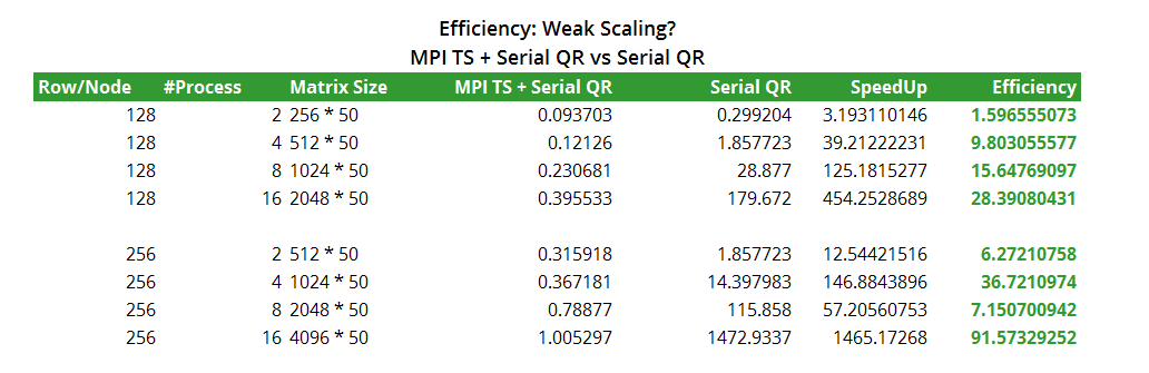
Keeping the work load per node constant, we test if the TSQR algorithm with Numpy QR is weak-scaling. Fixing the column number again, we tried different number of rows per node with P increasing from 2 to 8. The efficiency can be checked by the bar heights below. Disappointingly, there is no weak scaling for TSQR with Numpy.
Keeping the work load per node constant, we test if the TSQR algorithm with Numpy QR is weak-scaling. Fixing the column number again, we tried different number of rows per node with P increasing from 2 to 8. The efficiency can be checked by the bar heights below. Disappointingly, there is no weak scaling for TSQR with Numpy.
3. TSQR: MPI + Serial vs Serial
We then test the performance of TSQR with our self-implemented householder QR in Part 1. Gray figures in the chart below indicates a non-Tall-Skinny matrix, which will be rejected by the program.
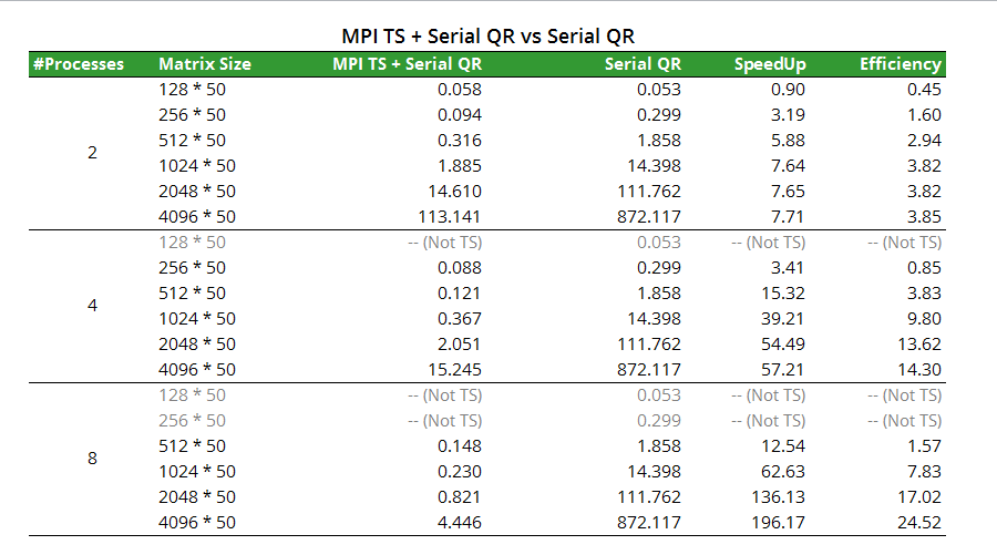
When analyzing efficiency in the same fashion as Part 2, we observed bizarre results. When taking a closer look into the design of TSQR algorithm, we found that the actual work load for TSQR is actually much lower compared to a serial QR thanks to the reduction. For example, when P processors and A is a m*n matrix with m > n, a serial QR needs to compute QR decomposition with O(m^3) complexity. However, a TSQR decomposes A into P (m/P) * n blocks, each with only O( (m/P) ^ 3) = O (m^3 / P^3) complexity, thus significantly reduces the work load.
The above reasoning can explain why we got efficiency far more than 1 - the way of efficiency calculation should be modified in analyzing TSQR algorithm. To conduct a fair comparison, one needs to work out the relationship between matrix size and the actual work load. Then choose the serial matrix size based on the latter. Due to time limit, we will leave this as a part of our future work.
The above reasoning can explain why we got efficiency far more than 1 - the way of efficiency calculation should be modified in analyzing TSQR algorithm. To conduct a fair comparison, one needs to work out the relationship between matrix size and the actual work load. Then choose the serial matrix size based on the latter. Due to time limit, we will leave this as a part of our future work.
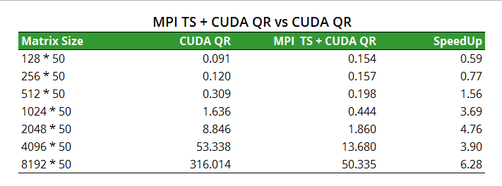
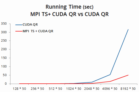
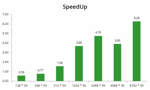
4. TSQR: MPI + CUDA vs CUDA
For MPI with CUDA QR, we can only use P = 2 as there are only two GPUs per node on the resonance cluster. It is a regret that we cannot do weak scaling due to this limit.
Again, we gain further speedup with matrix size increasing. For a matrix with size 4096 * 50, the figure is 3.9×. Together with the speedup we gained from using CUDA QR versus serial QR, our program enjoys a total speed up of 64×.
Again, we gain further speedup with matrix size increasing. For a matrix with size 4096 * 50, the figure is 3.9×. Together with the speedup we gained from using CUDA QR versus serial QR, our program enjoys a total speed up of 64×.
|
|
CS 205 Final Project | Fall 2013 | Xueshan Zhang and Ming Zhu
